
In our previous article, we discussed the concept of elliptic curves and the importance of homomorphic hiding in zero-knowledge proof systems. In this article, we will delve further into the polynomial specification process, which is another critical tool used in the core of zero-knowledge proofs.
Core Math Tools
1. Polynomial Specification Process
In the previous section, we discussed how homomorphic hiding allows for a non-interactive polynomial blind verification protocol, which is a crucial component of zero-knowledge proofs. Moving forward, we will explore the polynomial specification process in more detail. This involves using a series of mathematical tools, guided by Avi Wigderson’s zero-knowledge proof theory of NP problems and the theory of mutual specification of NP problems [6], to convert ordinary programs into polynomials.
1.1 Calculation Circuit
Let’s take this procedure as an example:
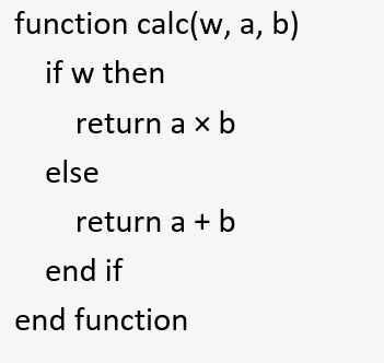
First we translate the program into a function expression:
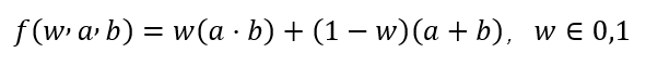
Consider this: any form of finite program can be expressed in this manner. For instance, both calc(1, 3, 2) and the evaluation of f(1, 3, 2) yield 6. Conversely, executing calc(0, 3, 2) and f(0, 3, 2) returns 5.
For our proof system, the objective is to prove that for the expression f(w, a, b) with input (1, 4, 2), the output is 8. In other words, Alice needs to demonstrate that she knows the value of (w, a, b) such that the polynomial expression:
w(a · b) + (1 – w)(a + b) = v, where w ∈ {0, 1}.
Let’s expand the function as follows:
w(a · b – a – b) + a + b = v
By doing so, we can simplify and flatten all the complex calculations into a calculation circuit.
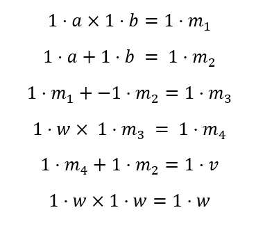
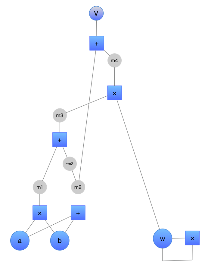
1.2 Gate Circuit Evaluation
Next, we will rely on polynomials to prove the correctness of a single calculation. The specific idea is as follows: To verify the correctness of a calculation, we must first ensure the correctness of the output/result obtained from the provided operands. We can represent each gate as an operational polynomial:
L(X) operator R(X) = O(X)
We can also define the following at some selected value ‘a’:
- l(x) represents the left operand’s value
- r(x) represents the right operand’s value
- o(x) represents the output/result of the operation
If both the operands and the result can be correctly represented in the form of a polynomial, then l(a) operator r(a) = o(a) can be considered true. In other words, if the value represented by the output polynomial o(x) is multiplied by the operators on the operand polynomials l(x) and r(x), the correct result of the operation is obtained.
To use this to our advantage, we can put the output polynomial o(x) to the left of the equation: l(a) operator r(a) – o(a) = 0
As long as the polynomial is valid, the operational polynomial must have a root ‘a’. Therefore, the polynomial must contain the factor (x – a), which is the target polynomial we will use for the proof, i.e., t(x) = x – a.
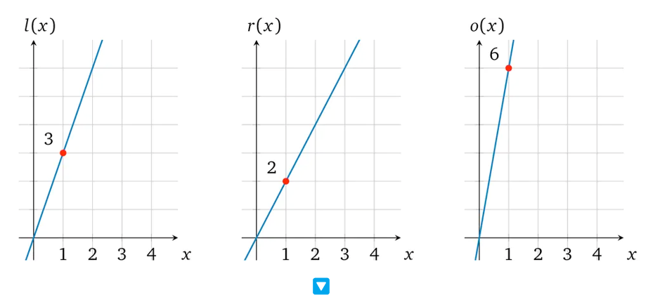
For example, let’s consider the operation 3×2=6. We can represent it with a simple polynomial:
- l(x) = 3x
- r(x) = 2x
- o(x) = 6x
Taking ‘a’ as 1, we get the following values:
- l(1) = 3
- r(1) = 2
- o(1) = 6
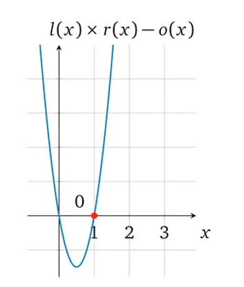
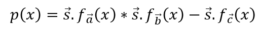
We can then obtain the image of p(x) = l(x) × r(x) – o(x):
- l(x) × r(x) = o(x)
- 3x × 2x = 6x
- 6x² – 6x = 0
- p(x) = 6x² – 6x
We have now transformed a multiplication gate calculation into a solution for the p(x) coefficient. While it is possible to solve for each gate in this way, it is not efficient. Therefore, in order to efficiently solve complex arithmetic circuits, we can use the idea of curve superposition.
Each gate circuit can be thought of as a curve that does not interfere with each other. If we superimpose all the gate circuits together, we can form a new curve that also does not interfere with each other at each gate solution. In this way, we can construct a curve and complete the calculation of all gates at once by solving the polynomial coefficients of this curve.
To construct such a curve, we introduce R1CS, which stands for Rank-1 Constraint System.
1.3 R1CS
To represent each gate circuit, we use an equivalent vector dot product process called Rank-1 Constraint System (R1CS).
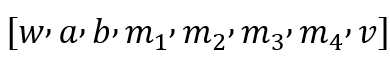
For each gate, we define a set of vectors
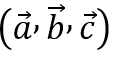
and a solution vector

(the vector of all inputs) such that
Each vector contains the input-output dimensions of all gates
and in order for the addition gate to be expressed in the same way, we add a dummy variable one, and the vector becomes:
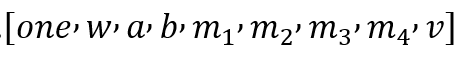
Corresponds to the first gate:
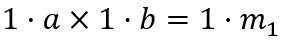
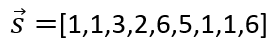
Solving the s vector represents all the inputs, outputs, and intermediate processes that satisfy the gate constraints. This is equivalent to knowing all the logic of the calc function, as well as the corresponding inputs and outputs.
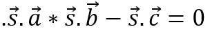
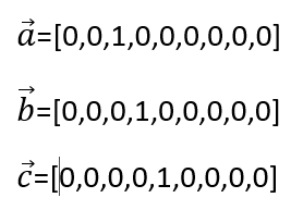
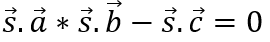
Substituting s, a, b, and c into s. a * s . b – s . c = 0 yields , where ⋅ represents the product of the vector
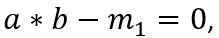
In other words, this vector expression is entirely equivalent to the first gate. The s vector that can satisfy the equation at this point is the solution to this gate circuit.
Using the same method, we can calculate each subsequent gate until we have represented the entire computational equation as a series of R1CS constraints.
The final solution we are looking for is the s-vector that satisfies all the R1CS constraints. This involves flattening the computation equation into a gate, and then encoding the gate into a vector expression using R1CS.
The next critical step involves representing the vector expression as a polynomial and finding the s-vector that satisfies all the constraints simultaneously. This process is known as Quadratic Arithmetic Programs (QAP).
1.4 QAP
The first step in QAP is to represent each dimension in the vector set we obtained in the section above
as the result of a polynomial:
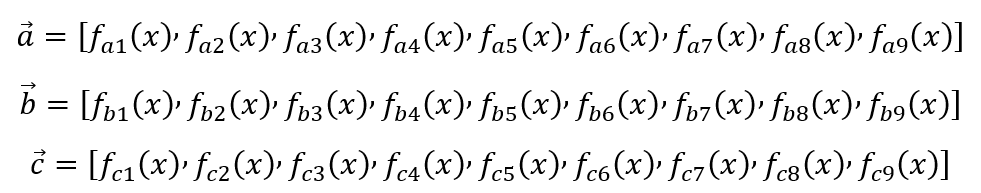
For each gate, we can make ‘x’ equal to a specific value:
- For Gate 1, ‘x’ is set to 1
- For Gate 2, ‘x’ is set to 2
- For Gate 3, ‘x’ is set to 3
- For Gate 4, ‘x’ is set to 4
- For Gate 5, ‘x’ is set to 5
- For Gate 6, ‘x’ is set to 6
Despite the different values of ‘x’, the R1CS vector dimensions remain the same for all gates.
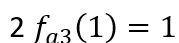
For example, if the third dimension of gate 1 takes a value of 1, then the

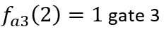
third dimension of gate
also has a value of

, then the third dimension of
takes value 0, then, by analogy, we can get
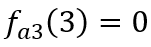
that this function is at

Given multiple points on a curve, how can we determine the curve? This requires the use of a mathematical tool called Lagrange interpolation, which is commonly used in universities. Anyone can use this tool to interpolate a polynomial.
In the second step, after we have obtained the polynomials of
substitute the

vectors to get the polynomial:
The preceding process shows that at x=1, x=2, x=3, x=4, x=5, x=6,
By using Lagrange interpolation, one can derive a polynomial that is determinatively divisible: t(x) = (x – 1)(x – 2)(x – 3)(x – 4)(x – 5)(x – 6).
In the third step, we can divide the polynomial and obtain h(x).
We have now transformed an ordinary computational program with branching conditions into a polynomial coefficient verification problem. From here, we can construct a non-interactive protocol for general zero-knowledge proofs using the homomorphic hiding algorithm introduced in Section 3.2.
The polynomial specification process involves two key mathematical ideas: constraint solving and hyperdimensionality. Through these concepts, we can catch a glimpse of the powerful thinking tools that mathematicians use to solve complex problems.
References
[6] Hartmanis J. Computers and intractability: a guide to the theory of np-completeness (michael r. garey and david s. johnson)[J]. Siam Review, 1982, 24(1): 90.